![[DL] Convolution and ReLU](https://img1.daumcdn.net/thumb/R750x0/?scode=mtistory2&fname=https%3A%2F%2Fblog.kakaocdn.net%2Fdn%2FzdMEO%2Fbtrw6gJ0SGb%2FbUskafRbjFh7TPQOfYzmbk%2Fimg.png)
1. Convolutional Base
합성곱 신경망(CNN)은 이미지에서 특징을 추출하는 convolutional base와 분류 작업을 하는 head로 구성되어 있다.
2. Feature Extraction
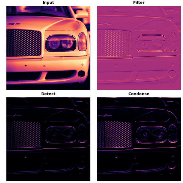
convolutional base는 convolution, ReLU, maximum pooling의 세 개의 작업으로 구성되어 있다. 이 세가지 단계는 각각의 작업을 수행한다.
- convolution : 이미지에서 특정 변수를 정제한다
- ReLU : 정제된 이미지에서 변수를 검사한다
- maximum pooling : 변수를 향상시키기 위해 이미지를 응축시킨다.
3. Filter with Convolution
convolutional layer는 필터링 단계를 수행한다. Keras 모델은 다음과 같이 코드를 작성하게 된다.
from tensorflow import Keras
from tensorflow.keras import layers

model = keras.Sequential([
	layers.Con2D(filter = 64, kernel_size = 3)
])
3.1 Weights
훈련과정에서 합성곱 신경망이 학습사는 가중치는 convolutional layer안에 포함되어 있는데, 이를 kernel이라고 부른다.
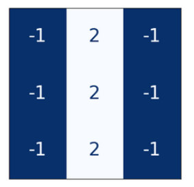
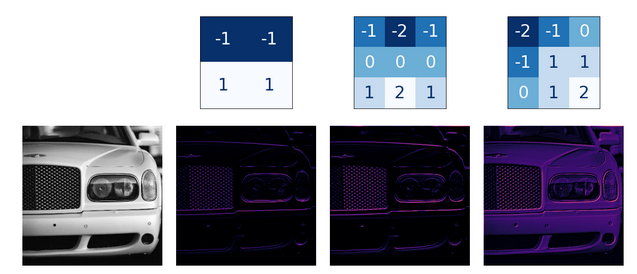
kernel은 이미지를 스킨하며 각 픽셀의 값에 가중합을 계산하게 된다. 즉, 편광렌즈처럼 작용하여 이미지의 패턴을 강조하거나 약화시킨다.
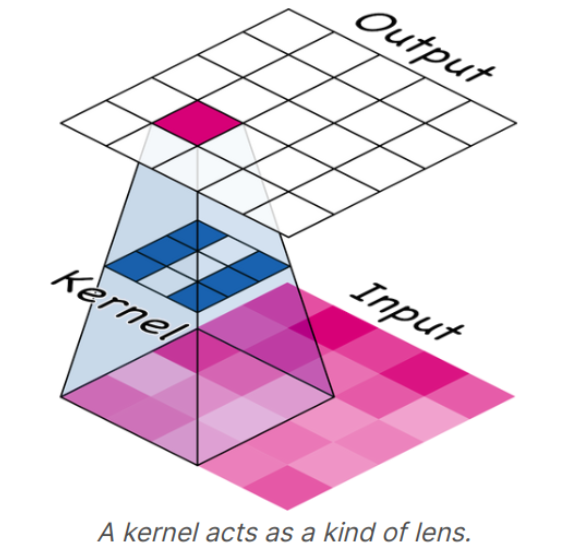
kernel은 어떻게 합성곱 신경망이 다음 layer에 연결될지를 정의한다. 즉 위의 사진에서 kernel의 결과물은 9개의 neuron의 input에 연결되며 kernel_size 파라미터를 통해 kernel 렌즈의 사이즈를 조정한다. 합성곱 신경망의 kernel은 어떤 종류의 변수들이 생성되는지 결정하게 되며 분류 문제를 위해 어떤 feature들이 필요하게 되는지 학습한다.
3.2 Activations
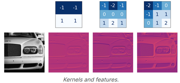
network의 활성화 함수는 feature map이라고 불린다. feature map은 생성된 filter를 이미지에 적용했을때 생성되는 결과로 kernel이 추출한 시각 변수를 포함하고 있다.
kernel 내부에 있는 숫자는 kernel이 생성하는 feature map을 정의하며, convolution이 강조하고 싶은 input값은 양의 값을 가지고 있다. filter 파라미터를 통해 합성곱 층이 얼마나 많은 feature map을 생성할 것인지를 결정하게 된다.
- feature : 생성하고자 하는 feature map의 수
- kernel_size : 커널 렌즈의 크기(홀수, 홀수)
3.3 Detect with ReLU
필터링 작업 이후에, feature map은 활성화 함수를 통과하게 된다. ReLU라고 불리는 활성화 함수는 Activation layer에 정의되며 활성화 함수를 픽셀 값에 중요도를 강조하게 된다. (음수값은 0)
4. Exercise(Filtering Image)
# Importing libraries

import tensorflow as tf
import matplotlib.pyplot as plt

# Visualization

plt.rc('figure', autolayout=True)
plt.rc('axes', labelweight='bold', labelsize='large',
       titleweight='bold', titlesize=18, titlepad=10)
plt.rc('image', cmap='magma')

# Importing dataset

image_path = '../input/computer-vision-resources/car_feature.jpg'
image = tf.io.read_file(image_path)
image = tf.io.decode_jpeg(image)

# Show image

plt.figure(figsize=(6, 6))
plt.imshow(tf.squeeze(image), cmap='gray')
plt.axis('off')
plt.show();

# Making kernel
# kernel using on example : edge detection

import tensorflow as tf

kernel = tf.constant([
    [-1, -1, -1],
    [-1,  8, -1],
    [-1, -1, -1],
])

plt.figure(figsize=(3, 3))
show_kernel(kernel)

# Reformat for batch compatibility.

image = tf.image.convert_image_dtype(image, dtype=tf.float32)
image = tf.expand_dims(image, axis=0)
kernel = tf.reshape(kernel, [*kernel.shape, 1, 1])
kernel = tf.cast(kernel, dtype=tf.float32)

# apply our kernel

image_filter = tf.nn.conv2d(
    input=image,
    filters=kernel,
    strides=1,
    padding='SAME',
)

# show filter

plt.figure(figsize=(6, 6))
plt.imshow(tf.squeeze(image_filter))
plt.axis('off')
plt.show();

# show the detected result

image_detect = tf.nn.relu(image_filter)

plt.figure(figsize=(6, 6))
plt.imshow(tf.squeeze(image_detect))
plt.axis('off')
plt.show();
5. Exercies : Convolution and ReLU
Step 1 : Define Kernel
# YOUR CODE HERE: Define a kernel with 3 rows and 3 columns.
kernel = tf.constant([
    [0, -1, 0],
    [-1, 5, -1],
    [0, -1, 0]
])
# Uncomment to view kernel
visiontools.show_kernel(kernel)
Step 2 : Apply Convolution
# YOUR CODE HERE: Give the TensorFlow convolution function (without arguments)
conv_fn = tf.nn.conv2d
Step 3 : Apply ReLU
# YOUR CODE HERE: Give the TensorFlow ReLU function (without arguments)
relu_fn = tf.nn.relu
'Course > [Kaggle] Data Science' 카테고리의 다른 글
| [DL] The Convolutional Classifier (0) | 2022.03.04 |
|---|---|
| [DL] Binary Classification (0) | 2022.03.02 |
| [DL] Dropout and Batch Normalization (0) | 2022.03.02 |
| [DL] Overfitting and Underfitting (0) | 2022.03.01 |
| [DL] Stochastic Gradient Descent (0) | 2022.03.01 |