![[DL] Overfitting and Underfitting](https://img1.daumcdn.net/thumb/R750x0/?scode=mtistory2&fname=https%3A%2F%2Fblog.kakaocdn.net%2Fdn%2FbJ72EX%2FbtruwJbrT1j%2FyKEz5Qz754Kl6wg3eUK3r0%2Fimg.png)
1. Interpreting the learning curve
강의에서는 훈련데이터의 정보를 Signal과 Noise로 분류한다. Signal은 데이터의 일반화된 부분이고, 새로운 데이터를 예측하는데 도움을 주는 부분이다. 반대로 Nosie는 훈련데이터의 실제의 값을 담당하며 모델의 예측에 크게 도움이 되지 않는 부분이다.
결국에 우리가 손실함수에 대한 Parameter와 weight를 최적화 시키더라도 궁극적으로는 새로운 데이터 즉, 평가 데이터에 대해 예측 정확도를 높여야 한다.
그래서 평가데이터에 대한 정확성을 훈련데이터의 정확성과 같이 플로팅하게 되는데 이것이 'Learning Curves'이다.
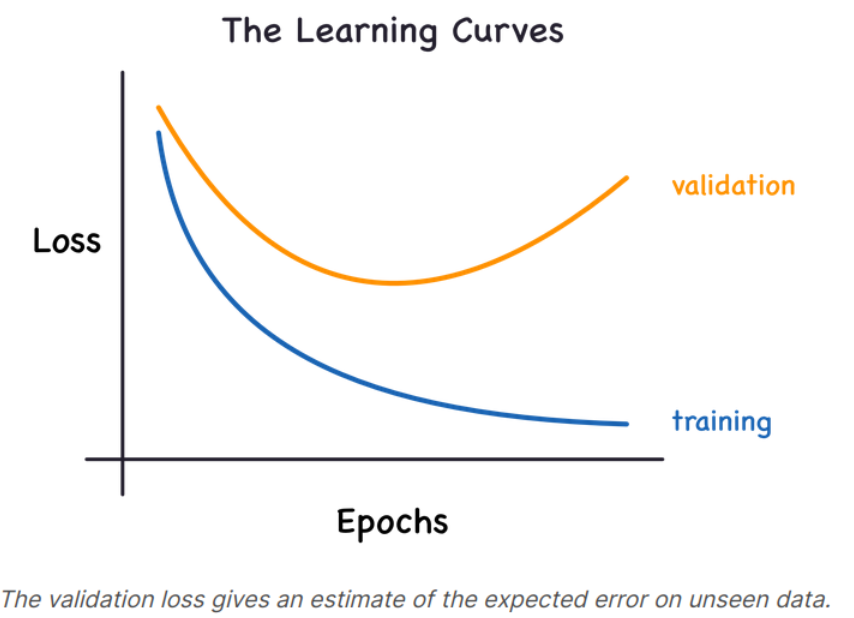
훈련 데이터의 손실함수 값은 Signal을 학습하던, Noise를 학습하던 지속적으로 감소한다. 하지만 평가 데이터의 손실함수 값은 Signal에 대해서만 학습할 때 감소한다. 위 그래프에서 Validation loss와 Training loss의 차이가 모델이 Noise를 학습하게 되는 정도가 된다.
이상적으로는 Signal만 학습하고 Noise를 배제하는 모델을 만들면 가장 좋으나 현실적으로는 불가능하다. 그래서 우리는 Signal을 최대한 학습하면서 Noise를 최대한 배제할 수 있는 최적점에서 학습하는 모델을 만들어야 한다. 즉. Validation loss가 증가하기 시작하는 지점이다.
2. Capacity
모델의 Capacity는 모델이 학습할 수 있는 사이즈와 복잡성을 의미한다. Neural Network에 대하여 이는 얼마나 많은 층이 쌓여 있거나, 뉴런이 존재하는지에 대해 결정된다. 그래서 만약 Neural Network가 Underfitting Problem이 존재한다면, Capacity를 증가시킴으로서 문제를 해결할 수 있다.
이 문제를 해결하는 방법은 각 층에 존재하는 neuron의 개수를 늘리는 방법과 층의 수를 늘리는 방법이 있다. 각각은 Wider network와 Deeper Network로, 전자는 선형 Underfitting Problem, 후자는 비선형 Underfitting Problem에 적용 가능하다.
model = keras.Sequential([
    layers.Dense(16, activation='relu'),
    layers.Dense(1),
])

wider = keras.Sequential([
    layers.Dense(32, activation='relu'),
    layers.Dense(1),
])

deeper = keras.Sequential([
    layers.Dense(16, activation='relu'),
    layers.Dense(16, activation='relu'),
    layers.Dense(1),
])
3. Early Stopping
Overfitting을 해결하는 방법은 Validation loss가 증가하기 시작할 때 모델의 훈련을 멈추는 방법이 있다. 즉, Validation loss의 기울기의 감소량이 줄기 시작하면 멈추면 된다. 이를 Early Stopping이라 한다.
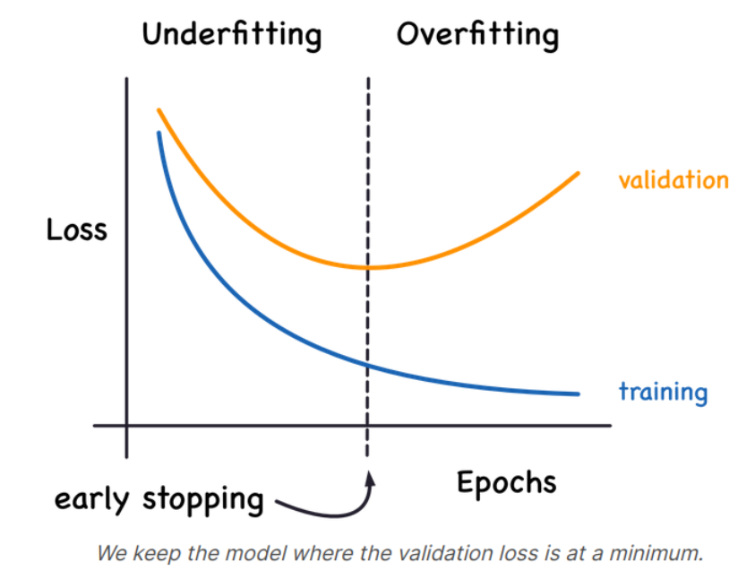
Validation loss가 다시 증가하기 시작하면 가중치를 다시 리셋하여 Model이 Overfit하는 것을 방지하게 된다. Early Stopping은 Model이 Overfitting하는 것 뿐만 아니라 Underfitting하는 것도 막아주게 된다(최소 기울기를 설정). 즉, 우리는 충분한 epoch만 공급하고 모델이 학습하도록 두면 된다.
4. Adding Early Stopping
Keras에서는 fitting을 할 때, callback을 통해 Early Stopping을 포함시키게 된다.
from tensorflow.keras.callbacks import EarlyStopping

early_stopping = EarlyStopping(
    min_delta=0.001, # minimium amount of change to count as an improvement
    patience=20, # how many epochs to wait before stopping
    restore_best_weights=True,
)- min_delta : Validation loss의 최소 상승 기울기
- patience : 기울기를 계산하기위한 epoch의 개수, iteration과는 다르다
5. Example
from tensorflow import keras
from tensorflow.keras import layers, callbacks

early_stopping = callbacks.EarlyStopping(
    min_delta=0.001, # minimium amount of change to count as an improvement
    patience=20, # how many epochs to wait before stopping
    restore_best_weights=True,
)

model = keras.Sequential([
    layers.Dense(512, activation='relu', input_shape=[11]),
    layers.Dense(512, activation='relu'),
    layers.Dense(512, activation='relu'),
    layers.Dense(1),
])
model.compile(
    optimizer='adam',
    loss='mae',
)

history = model.fit(
    X_train, y_train,
    validation_data=(X_valid, y_valid),
    batch_size=256,
    epochs=500,
    callbacks=[early_stopping], # put your callbacks in a list
    verbose=0,  # turn off training log
)
6. Exercise : Overfitting and Underfitting
Step 3 : Define Early Stopping Callback
model = keras.Sequential([
    layers.Dense(128, activation='relu', input_shape=input_shape),
    layers.Dense(64, activation='relu'),
    layers.Dense(1)
])
model.compile(
    optimizer='adam',
    loss='mae',
)
history = model.fit(
    X_train, y_train,
    validation_data=(X_valid, y_valid),
    batch_size=512,
    epochs=50,
    callbacks=[early_stopping]
)
history_df = pd.DataFrame(history.history)
history_df.loc[:, ['loss', 'val_loss']].plot()
print("Minimum Validation Loss: {:0.4f}".format(history_df['val_loss'].min()));
Source of the course : Kaggle Course _ Overfitting and Underfitting
Overfitting and Underfitting
Explore and run machine learning code with Kaggle Notebooks | Using data from DL Course Data
www.kaggle.com
'Course > [Kaggle] Data Science' 카테고리의 다른 글
| [DL] Binary Classification (0) | 2022.03.02 |
|---|---|
| [DL] Dropout and Batch Normalization (0) | 2022.03.02 |
| [DL] Stochastic Gradient Descent (0) | 2022.03.01 |
| [DL] Deep Neural Networks (0) | 2022.02.28 |
| [DL] A Single Neuron (0) | 2022.02.28 |