![[DL] Stochastic Gradient Descent](https://img1.daumcdn.net/thumb/R750x0/?scode=mtistory2&fname=https%3A%2F%2Fblog.kakaocdn.net%2Fdn%2FpLDfN%2FbtruI7P2TlJ%2FOEImuCA1dAhZlUDxv1z0J0%2Fimg.png)
1. Introduction
모델을 정의하는 것과는 별개로, 모델은 training data를 이용하여 학습되어야 한다. Neural Network는 예측값과 실제값의 차이가 가장 작은 가중치(weight)를 찾아야 한다.
- 손실함수(Loss Function) : 예측값과 실제값의 차이를 나타내는 함수
- Optimizer : 손실함수의 값을 최소화시키는 모델의 가중치를 찾는 방법
2. The Loss Function
손실함수(Loss Function)는 예측값과 실젯값의 분리도를 측정한다. 분류문제냐 회귀문제냐에 따라 손실함수가 달라지게 되는데, 회귀 문제에서는 연속형 값을 손실함수에 적용한다. 회귀문제에서 흔히 사용하는 손실함수는 Mean Absoulte Error(MAE)로, 예측값과 관측값의 차이에 대하여 절댓값의 평균을 계산한다.
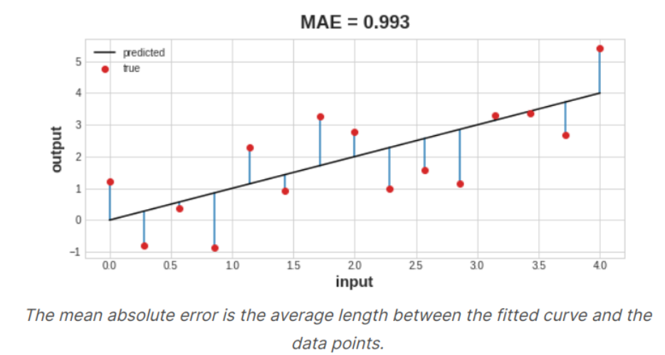
훈련을 진행하면서, 모델은 손실함수를 사용하여 최적의 가중치를 찾는데 도움을 얻을 수 있다.
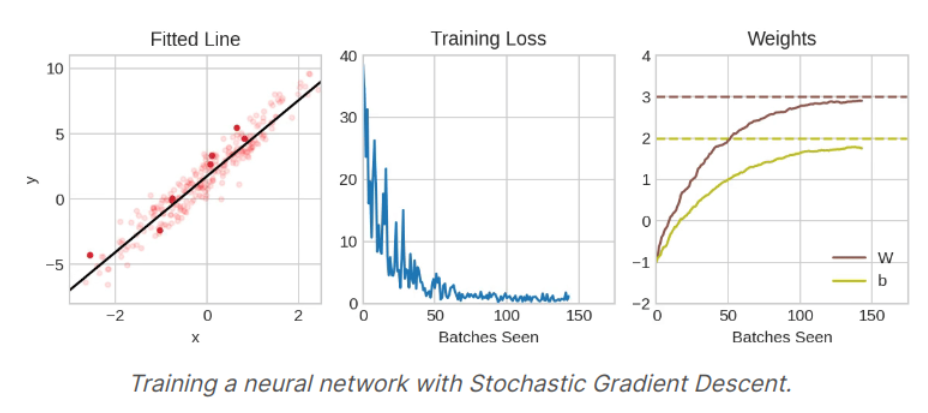
3. The optimizer - Stochastic Gradient Descent
손실함수를 계산할 수 있지만, 손실함수를 최소화하는 방법은 아직 정의되지 않았다. 이때 등장하는 개념이 Optimizer로, Optimizer는 손실함수를 최소화하는 모델의 가중치를 계산하게 된다.
딥러닝에서 사용되는 모든 최적화 알고리즘은 '확률적 경사 하강법'(Stochastic Gradient Descent; SGD)라고 하며, 반복적으로 단계를 수행하며 진행되는 알고리즘이다.
- 훈련데이터에서 몇개의 샘플을 추출한 뒤, Neural Network에 적용시켜 예측을 수행한다.
- 예측값과 관측값의 차이를 손실함수를 이용하여 계산한다
- 그 뒤 손실함수의 값을 최소화시키는 가중치의 방향을 정한 후 계속 반복한다
이 과정을 손실함수의 값이 최소화 될 때까지 진행하며, 각각의 훈련에 사용되는 데이터 샘플을 미니배치(mini batch)라고 한다. 더불어 Neural Network에서 입력부터 출력까지 각 계층의 가중치(weight)를 계산하는 순방향 전파(Feed Forward process)와 반대로 거슬러 올라가며 기존의 가중치(weight)를 수정하는 역전파(Back Propagation)가 완료되는 과정을 epoch라고 한다.
4. Learning Rate and Batch Size
epoch와 mini batch의 사이즈는 SGD알고리즘의 가장 중요한 초매개변수(Hyperparameter)로, mini batch 데이터셋의 개수에 따라 iteration이 발생하며, 이 iteration과 epoch의 곱이 총 진행된 학습의 횟수이다.
Fortunately, for most work it won't be necessary to do an extensive hyperparameter search to get satisfactory results. Adam is an SGD algorithm that has an adaptive learning rate that makes it suitable for most problems without any parameter tuning. Adam is great general-purpose optimizer.
5. Adding the Loss and Optimizer
미리 정의된 model에 compile method를 사용하여 optimizer과 loss function을 지정해 줄 수 있다.
model.compile(
    optimizer = "adam",
    loss = "mae"
)
6. Example
import pandas as pd
from IPython.display import display

red_wine = pd.read_csv('../input/dl-course-data/red-wine.csv')

# Create training and validation splits
df_train = red_wine.sample(frac=0.7, random_state=0)
df_valid = red_wine.drop(df_train.index)
display(df_train.head(4))

# Scale to [0, 1]
max_ = df_train.max(axis=0)
min_ = df_train.min(axis=0)
df_train = (df_train - min_) / (max_ - min_)
df_valid = (df_valid - min_) / (max_ - min_)

# Split features and target
X_train = df_train.drop('quality', axis=1)
X_valid = df_valid.drop('quality', axis=1)
y_train = df_train['quality']
y_valid = df_valid['quality']


# Define a model

from tensorflow import keras
from tensorflow.keras import layers

model = keras.Sequential([
    layers.Dense(512, activation='relu', input_shape=[11]),
    layers.Dense(512, activation='relu'),
    layers.Dense(512, activation='relu'),
    layers.Dense(1),
])

model.compile(
    optimizer='adam',
    loss='mae',
)

# This will show the changes of loss

history = model.fit(
    X_train, y_train,
    validation_data=(X_valid, y_valid),
    batch_size=256,
    epochs=10,
)

# convert the training history to a dataframe

history_df = pd.DataFrame(history.history)

# use Pandas native plot method

history_df['loss'].plot();
7. Exercise : Stochastic Gradient Descent
Step 1 : Add Loss and Optimizer
# YOUR CODE HERE
model.compile(
    optimizer = 'adam',
    loss = 'mae'
)
Step 2 : Train Model
# YOUR CODE HERE
history = model.fit(
    X, y,
    batch_size = 128,
    epochs = 200
)
Souce of the course : Kaggle Course _ Stochastic Gradient Descent
Stochastic Gradient Descent
Explore and run machine learning code with Kaggle Notebooks | Using data from DL Course Data
www.kaggle.com
'Course > [Kaggle] Data Science' 카테고리의 다른 글
| [DL] Dropout and Batch Normalization (0) | 2022.03.02 |
|---|---|
| [DL] Overfitting and Underfitting (0) | 2022.03.01 |
| [DL] Deep Neural Networks (0) | 2022.02.28 |
| [DL] A Single Neuron (0) | 2022.02.28 |
| [SQL] Writing Efficient Queries (0) | 2022.02.24 |