![[SQL] Writing Efficient Queries](https://img1.daumcdn.net/thumb/R750x0/?scode=mtistory2&fname=https%3A%2F%2Fblog.kakaocdn.net%2Fdn%2FbtefGD%2FbtruiQ1VrKI%2FdUCtpxKC3DfnaTnb2zUPk0%2Fimg.png)
1. Some useful functions
- show_amount_of_data_scanned() shows the amount of data the query uses
- show_time_to_run() prints how long it takes for the query to execute
from google.cloud import bigquery
from time import time

client = bigquery.Client()

def show_amount_of_data_scanned(query):
    # dry_run lets us see how much data the query uses without running it
    dry_run_config = bigquery.QueryJobConfig(dry_run=True)
    query_job = client.query(query, job_config=dry_run_config)
    print('Data processed: {} GB'.format(round(query_job.total_bytes_processed / 10**9, 3)))

def show_time_to_run(query):
    time_config = bigquery.QueryJobConfig(use_query_cache=False)
    start = time()
    query_result = client.query(query, job_config=time_config).result()
    end = time()
    print('Time to run: {} seconds'.format(round(end-start, 3)))
2. Strategies
- Only select the columns you want
It is tempting to start queries with SELECT * FROM ... it's convinient because you don't need to think about which columns you need. But it can be very inefficient.
This ise especially important if there are text fields that you don't need, because text field tend to be larger than other fields.
star_query = "SELECT * FROM `bigquery-public-data.github_repos.contents`"
show_amount_of_data_scanned(star_query)

basic_query = "SELECT size, binary FROM `bigquery-public-data.github_repos.contents`"
show_amount_of_data_scanned(basic_query)
In this case, we see a 1000X reduction in data being scanned to complete the query, because the raw data contained a text field that was 1000X larger than the fields we might need.
- Read less data
Both queries below calculate the average duration (in seconds) of one-way bike trips in the city of San Francisco.
more_data_query = """
                  SELECT MIN(start_station_name) AS start_station_name,
                      MIN(end_station_name) AS end_station_name,
                      AVG(duration_sec) AS avg_duration_sec
                  FROM `bigquery-public-data.san_francisco.bikeshare_trips`
                  WHERE start_station_id != end_station_id
                  GROUP BY start_station_id, end_station_id
                  LIMIT 10
                  """
show_amount_of_data_scanned(more_data_query)

less_data_query = """
                  SELECT start_station_name,
                      end_station_name,
                      AVG(duration_sec) AS avg_duration_sec
                  FROM `bigquery-public-data.san_francisco.bikeshare_trips`
                  WHERE start_station_name != end_station_name
                  GROUP BY start_station_name, end_station_name
                  LIMIT 10
                  """
show_amount_of_data_scanned(less_data_query)
Since ther is a 1:1 relationship between the station ID and the station name, we don't need to use the 'start_station_id' and 'end_station_id' columns in the query. By using only the columns with the station IDs, we can less data.
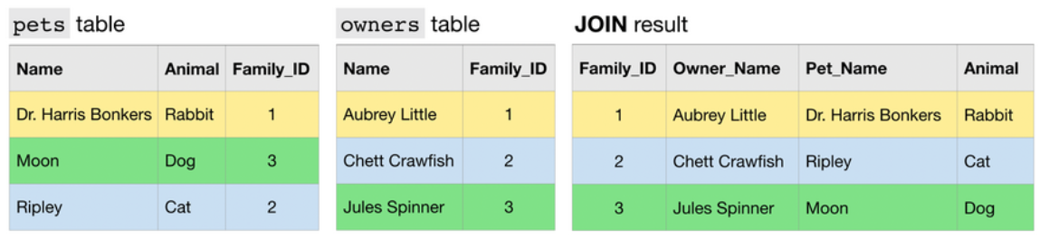
- Avoid N:N JOINs
Most of JOINs that we have executed in the course have been 1:1 JOINs.
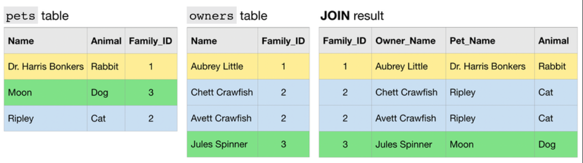
Another type of JOIN is an N:1 JOIN. Here, each row in one table matches potentially many rows in the other table.
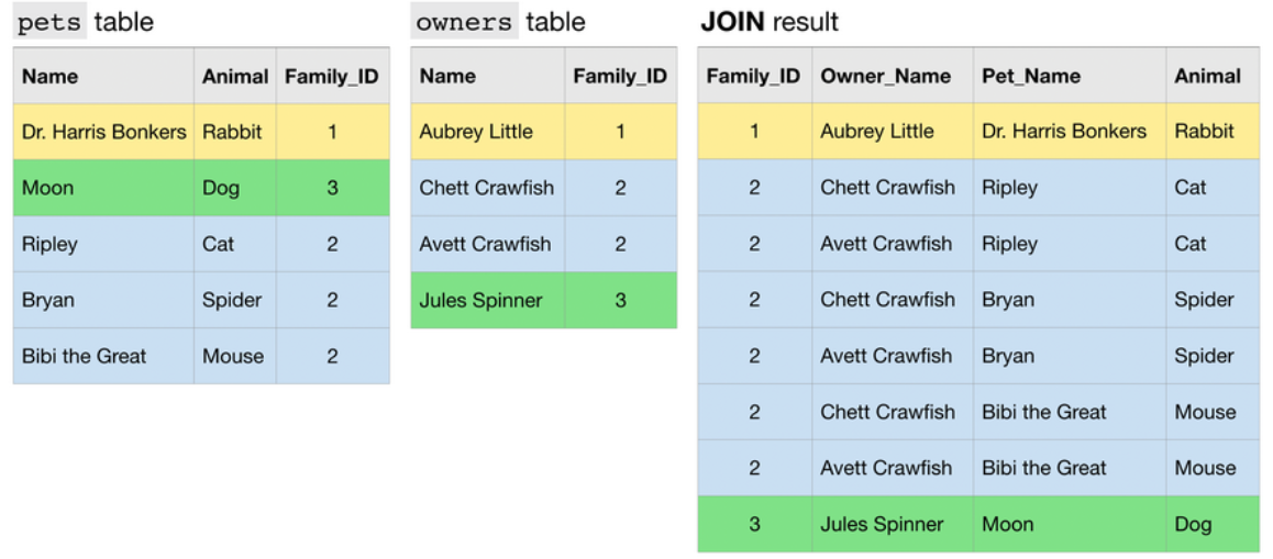
Finally, an N:N JOIN is one where a group of rows in one table can match a group of rows in the other table. Note that in general, all other things equal, this type of JOIN produces a table with many rows than either of the two tables that are being JOINed.
big_join_query = """
                 SELECT repo,
                     COUNT(DISTINCT c.committer.name) as num_committers,
                     COUNT(DISTINCT f.id) AS num_files
                 FROM `bigquery-public-data.github_repos.commits` AS c,
                     UNNEST(c.repo_name) AS repo
                 INNER JOIN `bigquery-public-data.github_repos.files` AS f
                     ON f.repo_name = repo
                 WHERE f.repo_name IN ( 'tensorflow/tensorflow', 'facebook/react', 'twbs/bootstrap', 'apple/swift', 'Microsoft/vscode', 'torvalds/linux')
                 GROUP BY repo
                 ORDER BY repo
                 """
show_time_to_run(big_join_query)

small_join_query = """
                   WITH commits AS
                   (
                   SELECT COUNT(DISTINCT committer.name) AS num_committers, repo
                   FROM `bigquery-public-data.github_repos.commits`,
                       UNNEST(repo_name) as repo
                   WHERE repo IN ( 'tensorflow/tensorflow', 'facebook/react', 'twbs/bootstrap', 'apple/swift', 'Microsoft/vscode', 'torvalds/linux')
                   GROUP BY repo
                   ),
                   files AS
                   (
                   SELECT COUNT(DISTINCT id) AS num_files, repo_name as repo
                   FROM `bigquery-public-data.github_repos.files`
                   WHERE repo_name IN ( 'tensorflow/tensorflow', 'facebook/react', 'twbs/bootstrap', 'apple/swift', 'Microsoft/vscode', 'torvalds/linux')
                   GROUP BY repo
                   )
                   SELECT commits.repo, commits.num_committers, files.num_files
                   FROM commits
                   INNER JOIN files
                       ON commits.repo = files.repo
                   ORDER BY repo
                   """

show_time_to_run(small_join_query)
3. Exercise : Writing Efficient Queries
Step 1 : You work for Pet Costumes International
# Fill in your answer
query_to_optimize = 3
Step 2 : Make it easier to find Mitzie!
WITH CurrentOwnersCostumes AS
(
SELECT CostumeID
FROM CostumeOwners
WHERE OwnerID = MitzieOwnerID
),                                # CostumeOwner에서 MitzieOwnerID를 먼저 추출하여 1번 전략 이행
OwnersCostumesLocations AS
(
SELECT cc.CostumeID, Timestamp, Location
FROM CurrentOwnersCostumes cc INNER JOIN CostumeLocations cl
    ON cc.CostumeID = cl.CostumeID
),                                # 선택한 CostumeID 와 동일한 ID를 CostumeLocations에서 Timestamp, Location 추출
LastSeen AS
(
SELECT CostumeID, MAX(Timestamp)
FROM OwnersCostumesLocations
GROUP BY CostumeID
)                                # 선택된 dataset에서 Timestamp의 MAX값 추출 -> 최근값 저장
SELECT ocl.CostumeID, Location
FROM OwnersCostumesLocations ocl INNER JOIN LastSeen ls
    ON ocl.timestamp = ls.timestamp AND ocl.CostumeID = ls.costumeID

# OwnerCostumesLocation(Mitzie의 펫에 대한 정보를 기록하고 있는 데이터셋에서 LastSeen에 저장한 최근값을 비교하여 위치 선택
Source of the course : Kaggle Course _ Writing Efficient Queries
'Course > [Kaggle] Data Science' 카테고리의 다른 글
| [DL] Deep Neural Networks (0) | 2022.02.28 |
|---|---|
| [DL] A Single Neuron (0) | 2022.02.28 |
| [SQL] Nested and Repeated Data (0) | 2022.02.24 |
| [SQL] Analytic Functions (0) | 2022.02.24 |
| [SQL] JOINs and UNIONs (0) | 2022.02.24 |